In this post I want to go over the three main strategies of resolution that are popular in the modern day. Both for general knowledge-sharing, but also because I think SLG resolution might be useful when thinking about the AVM.
But first of all, for those not in the know- what do we mean by ‘resolution’? Resolution calculus is a formalisation of first-order logic inference systems. To ‘resolve’ means to ‘infer’. Each of these resolution systems can thus be described by the same calculus, with the same elements, but different control strategies:
- Horn Clauses
Any formal description of what a ‘horn clause’ is in FOL is out of scope. What I mean by a ‘horn clause’ is a statement of the type
Goal :- Subgoal1, Subgoal2...
WhereGoalis a term we are trying to prove (called a ‘positive literal’) andSubgoal1,Subgoal2are its subterms which must be evaluated and proven to show thatGoalis true.
Each term looks like
Predicate(Var1, Var...)
wherePredicatemay be any symbol we like, and eachVarcould be a constant (E.G., a string, a number, an atom) or some arbitrary symbol preprended with a capital letter such asX,Sym, etc- which symbolises something we have yet to infer the meaning of. It can also refer to compound data types lists["blah", 1, 2]- or even terms themselves (though these remain unevaluated unless specifically called during the program’s run).
It’s important to note that a horn clause can have no subterms, in which case the goal is unconditionally true.
- A Database*
A database is a store of horn clauses.
For example I might write a stupid program
actor(john).
actor(jill).
rich(X) :- actor(X).
All of these are horn clauses (simply stating a(1). means it is a goal with no subterms).
Each horn clause is stored in the database by my program. These clauses can then be accessed at query time (something we’ll get to in a moment).
- Unification
This is the primary method of resolving symbols. If I write a casual statement
X = 4 obviously this means that the value of the symbol X should be bound to 4. We say X has been ‘unified’ with 4.
If I write even(X), divides_by_four(X), X = 4. as a couple of subclauses then I should expect that all X in the statement will be equivalent- they will be unified.
We can also unify terms.
int(X) = int(4) in which case X will be bound to 4. Unification can be arbitrarily deep and works on any data structure.
- Queries*
A query looks like
?- factorial(X, Z), X = 5, more_than_100(Z).
It is a ?- followed by a list of terms which represent goals. When a query is executed, the program will attempt to infer that the goals are true, unifying any symbols in the process and providing their values.
For example we would expect
?- factorial(X, 120). to unify X with 5.
How does it actually infer that information? Well that depends on the resolution strategy, but it invariably involves unifying these goals with some information in the database, and forming a chain of subgoals.
(* Datalog works a little different to PROLOG on these points. But we’ll get to that.)
SLD Resolution
This is the essential model of PROLOG. The ‘SLD’ stands for:
Selective → At each step, pick one singular subgoal to resolve out of a candidate list.
Linear → Pick the latest subgoal to resolve on.
Definite → No disjunctions in the head- I.E., there can only be one term in the goal of each clause (don’t worry about this one, we won’t get onto things like disjunctive heads, they surprisingly aren’t very useful anyway. But know that in certain languages you can have statements of the form P, Q :- Subterm. which denote that if Subterm holds, then either P or Q hold).
Easy mnemonic for you. But what does this actually mean? The easiest way to explain is with this classic example.
parent(john, jack).
parent(john, jill).
parent(james, john).

ancestor(X, Z) :- parent(X, Z).
ancestor(X, Z) :- parent(X, Y), ancestor(Y, Z).
This program states that John is the parent of Jack, and of Jill. It also states that James is a parent of John. Simple base facts. No subterms.
The ancestor clause is more interesting. For X to be an ancestor of Z is either to mean that X is a direct parent of Z or that X is a parent of Y, and Y is an ancestor of Z. Take a second to reason out for yourself that this logically must cover all possible cases.
What happens if I query ?- ancestor(X, Z).? The first thing that happens is a unification the goals in the head in the database- that is, two clauses are found to match a statement of this pattern:
ancestor(X, Z) :- parent(X, Z).
ancestor(X, Z) :- parent(X, Y), ancestor(Y, Z).
Next, the first clause is selected, and its body- parent(X, Z), is treated as a new subgoal. This most recently selected subgoal is now itself unified with the database to yield
parent(john, jack).
parent(john, jill).
parent(james, john).
and parent(john, jack) is picked. X and Z therefore become unified with john and jack respectively. And this is our first query result
?- ancestor(X, Z).
X = john,
Z = jack.
However, PROLOG won’t just return one answer. It will return all answers, by use of something called a ‘choicepoint’. This whole time, PROLOG wasn’t only going through a chain naively- it was also creating a stack of decisions and other possible decisions that it could have made. That means that we can also return the next answer that would have been returned if parent(john, jack) didn’t exist- and by that method, we can get all of the answers, in order.
?- ancestor(X, Z).
X = john,
Z = jack ;
X = john,
Z = jill ;
X = james,
Z = john ;
X = james,
Z = jack ;
X = james,
Z = jill.
This kind of program is called exhaustive- all answers will eventually be found.
Our program is also complete- if there is an answer, it will eventually be found.
Finally, it is bidirectional- we can query both ancestor(john, Z) and ancestor(X, jack) and in both cases expect answers- this means PROLOG is excellent for both generating as well as testing.
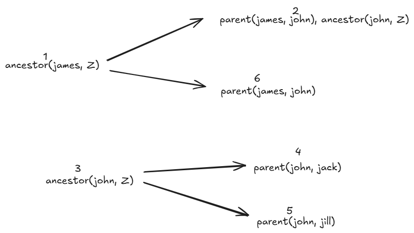
If you still don’t get it- consult the following tree, and you surely will understand. The numbers denote order of answer.

In a sentence, SLD resolution is a depth-first search of the tree of all possible answers to my query.
‘Bottom-Up Execution’ AKA Datalog
Sometimes the PROLOG execution strategy is called ‘backwards-chaining’ because you go ‘backwards’ from the goal to the leaves of the tree in order to prove the goal. Do you think maybe we can also go in the other direction? I.E., start from the base facts and compute all possible new facts? Yes we can!
Now to address the asterisk from earlier. Datalog is not really the same as these other two. The ‘database’ in datalog is actually two databases- an intensional database, and an extensional database.
We start from an extensional database of ground terms (no vars, no subgoals). You’ll often see this concept referred to as a ‘Herbrand Base’.
parent(john, jack).
parent(john, jill).
parent(james, john).
and add to it an intensional database of clauses we want to derive new facts from.
ancestor(X, Z) :- parent(X, Z).
ancestor(X, Z) :- parent(X, Y), ancestor(Y, Z).
All of the hard work actually occurs when the IDB and EDB are brought together, and not during the query. Datalog evaluation is described usually in ‘rounds’. In round 1, all of the EDB facts fire, and a clause is selected for each.
In round 1, we will get these new terms:
ancestor(john, jack).
ancestor(john, jill).
ancestor(james, john).
This is because the second ancestor/2 clause involves there being ancestor/2 base facts having been discovered- there aren’t any.
On round 2, though, we get
ancestor(james, jack).
ancestor(james, jill).
Because we were able to use the facts from round 1 to discover new facts.
Once no new facts are found in a round, the work is complete. We have reached what is called a fixpoint. This strategy ensures completion.
Finally, the user can query the resulting database, which just involves naive unification of all the ground facts.
?- ancestor(james, jill).
true
Only new facts are ever found, not deleted, meaning datalog is monotonic. This is one reason why it has been popular amongst the Clojure crowd, as seen from Datomic and XTDB v1.
There are two more things about datalog.
- There cannot be arbitrarily nested terms such as
f(f(f(1))). - Only finite domains can be operated upon (no arbitrary ints)
It is not Turing-complete. Evaluation will eventually end.
SLG Resolution.
The imaginative reader will already be making many considerations and asking intelligent questions- such as: Why can’t we memoise subgoals in PROLOG? What about if we did a breadth-first search instead? Can we do concurrent search? How can we handle loops? How can we make it smarter, without losing expressiveness? How do we handle negation?
Whilst there are strategies for avoiding loops, memoisation, and for breadth-first search, it must be admitted that all of these questions are nonetheless valid. They have haunted PROLOG engineers for a generation, and the concurrency problem specifically was the catalyst for its evolution into Erlang.
SLG Resolution, in my opinion, is one of the most promising options for a read-heavy, monotonic system and I’ve been fascinated by it recently, and was the inspiration to even make this post, since I think it could be influential on the AVM.
The S & L mean selective and linear, like with SLD resolution, but the ‘G’ stands for ‘general’. What is this generality?
According to Chen & Warren, SLG is a ‘partial deduction system’ and
Rather than detecting and handling infinite recursion through negation, we focus on the complementary problem of ensuring the complete evaluation of subgoals.
(...)
SLG resolution allows a programmer or an implementer to choose an arbitrary computation rule for selecting a literal from a rule body and to choose an arbitrary strategy for selecting which transformation to apply.
(...)
SLG resolution supports answer sharing of subgoals that are variants of each other. A subgoal is guaranteed to be evaluated only once.
(...)
SLG resolution delays ground negative literals that are involved in a loop and simplified them away when their truth values become known to be true or fake. The delaying mechanism is the key to the maximum freedom in control strategies and enables SLG resolution to avoid the repetition of any derivation step.
Well that sounds lovely. The paper itself is quite complex and mathsy, but I can break it down for you in a simple way.
At the most horribly oversimplified level, SLG resolution simply tables subgoals and their answers.
As with SLD, we have a global database of clauses
parent(john, jack).
parent(john, jill).
parent(james, john).

ancestor(X, Z) :- ancestor(Y, Z), parent(X, Y).
ancestor(X, Z) :- parent(X, Z).

:- table ancestor/2.
Note here that the first ancestor clause has its subgoals flipped from before, which in SLD should cause infinite recursion.
Now I call ?- ancestor(james, Z). First, it has been recorded that ancestor/2 is a table. A table is created now. But I must tell you that this table does not necessarily specifically mean only a table for ancestor/2- by default in XSB PROLOG for example, there is something called ‘variant tabling’, which means that a table specifically for ancestor(james, Z) is what was also created. Later if there is a call ancestor(X, Z), it may take answers from the ancestor/2 table (this is called subsumption tabling), but also create its own table. All of these details of tables can be managed by the user.
ancestor(X,Z) :- ancestor(X,Y), parent(Y,Z).
ancestor(X,Z) :- parent(X,Z).
Now when the first clause resolves to ancestor(X, Y), it sees that a table exists already of the form ancestor(X, Y) without answers and suspends this computation, and instead looks towards the second, finding all the immediate answers.
ancestor(james, john).
And only then will the first computation resume, now unblocked finding the rest.
However, if we look at a right-recursive example,
parent(john, jack).
parent(john, jill).
parent(james, john).

ancestor(X, Z) :- parent(X, Y), ancestor(Y, Z).
ancestor(X, Z) :- parent(X, Z).

:- table ancestor/2.
If we query again ancestor(james, Z), then what I hope you are able to see will happen is an extra table will be found: ancestor(john, Z). The result will be the same, but it required an extra table. We say that SLG-resolution resolves on a forest whereas SLD-resolution resolves on a tree.
Suppose that there is a mutual dependency between these two trees? In this case, the two trees are marked as a ‘strongly connected component’ or ‘SCC’. SCCs must be completed as a unit.
Updates can be strange here, but for monotonic programs, you can run incremental tabling, which means that new facts precipitate down by pushing deltas to the relevant tables, with workers processing those deltas.
Yes, workers. One great thing about all this is you can make everything concurrent. Tables can be seen as long-running processes in communication with their dependents. The work of both sides of the ancestor/2 clause could take place at once (until the first has to pause and wait for the second). In this way, SLG resolution really is ‘logical erlang’. And if you want SLD, just don’t tell it to make tables!
The only implementation of a proper SLG resolver I know of is XSB PROLOG, but I feel that it is much too important to leave out here. I find SLG resolution highly promising for concurrent machines. One nice thing about XSB btw is that it is almost identical in interface to SWI-PROLOG, so it regularly has stuff ported over like constraint-processing libraries.
Addendum
Lastly, you can always make for yourself a specialised resolver. As you’ve seen with SLG, we can put information around clauses to change control flow details (this should be reminiscent of the MOP). But I have written enough and will leave this as an exercise for the reader.